inamerrata

Things are different now. That’s certain.

Or at least that’s what one of the marketing sites for my new employer has to say.

Back in March I started at Red Hat’s Brisbane office working in release engineering (or the “Release Configuration Management” team). Short summary: it’s been pretty fun so far.

Googling just now for something to link that provides some sort of context, I came upon a video with my boss (John Flanagan) and one of my colleagues (Jesse Keating) — neither of whom I’ve actually met yet — giving a talk to the ACM chapter at Northeastern University in Boston. (It’s an hour long, and doesn’t expect much background knowledge of Linux; but doesn’t go into anything in any great depth either)

My aim in deciding to go job hunting late last year was to get a large change of scenery and get to work with people who understood what I was doing — it eventually gets a bit old being a black box where computer problems go in, solutions come out, and you can only explain what happens in between with loose analogies before seeing eyes glaze over. Corporate environment, Fedora laptop, enterprise customers, and a zillion internal tools that are at least new to me, certainly counts as a pretty neat change of scenery; and I think I’ve now got about five layers of technical people between me and anyone who doesn’t have enough technical background to understand what I do on the customer side. Also, money appears in my bank account every couple of weeks, without having to send anyone a bill! It’s like magic!

The hiring process was a bit odd — mostly, I gather, because while I applied for an advertised position, the one I ended up getting was something that had been wanted for a while, but hadn’t actually had a request open. So I did a bunch of interviews for the job I was applying for, then got redirected to the other position, and did a few interviews for that without either me or the interviewers having a terribly clear idea what the position would involve. (I guess it didn’t really help that my first interview, which was to be with my boss’s boss, got rearranged because he couldn’t make it in due to water over the roads, and then Brisbane flooded; that the whole point of the position is that they didn’t have anyone working in that role closer than the Czech Republic is probably also a factor…)

As it’s turned out, that’s been a pretty accurate reflection of the role: I’ve mostly been setting my own priorities, which mostly means balancing between teaching myself how things work, helping out the rest of my team, and working with the bits of Red Hat that are local, or at least operate in compatible timezones. Happily, that seems to be working out fairly okay. (And at least the way I’ve been doing it isn’t much different to doing open source in general: “gah, this program is doing something odd. okay, find the source, see what it’s doing and why, and either (a) do something different to get what you want, or (b) fix the code. oh, and also, you now understand that program”)

As it turned out, that leads into the main culture shock I had on arriving: what most surprised me was actually the lack of differences compared to being involved in Debian — which admittedly might have been helped by a certain article hitting LWN just in time for my first day. “Ah, so that list is the equivalent of debian-devel. Good to know.” There’s a decent number of names that pop up that are familiar from Debian too, which is nice. Other comfortingly familiar first day activities were subscribing to more specific mailing lists, joining various IRC channels, getting my accounts setup and setting up my laptop. (Fedora was suggested, “not Debian” was recommended ;)

Not that everything’s the same — there’s rpm/yum versus dpkg/apt obviously, and there’s a whole morass of things to worry about working for a public company. But a lot of it fits into either “different to Debian, but not very” and “well, duh, Red Hat’s a for-profit, you have to do something like this, and that’s not a bad way of doing it”.

Hmm, not sure what else I can really talk about without at least running it by someone else to make sure it’s okay to talk about in public. I think there’s only a couple of things I’ve done so far that have gone via Fedora and are thus easy — the first was a quick python script to make publishing fedora torrents easier, and the other was a quick patch to the fedora buildsystem software to help support analytics. Not especially thrilling, though. I think Dennis is planning on throwing me into more Fedora stuff fairly soon, so hopefully that might change.

Reading through some of the comments from last year’s Linux Australia Survey, a couple struck me as interesting. One’s on Java:

linux.conf.au seems to have a bias against Java. Since Java is an open source language and has a massive open source infrastructure, this has not made a lot of sense to me. It seems that Python, Perl, PHP, Ruby are somehow superior from an open source perspective even though they are a couple of orders of magnitude less popular than Java in the real world. This bias has not changed since openjdk and I’m guessing is in the DNA of the selectors and committee members. Hence *LUG* has lost a lot of appeal to me and my team. It would be good if there was an inclusive open source conference out there…

and the other’s more general:

I appreciate LCA’s advocacy of open source, but I feel that a decoupling needs to be made in the mindshare between the terms “open source” and “Linux”. Unfortunately, for people involved in open source operating systems that aren’t Linux, we may feel slightly disenfranchised by what appears to be a hijacking of the term “open source” (as in “the only open source OS is linux” perception).

My impression is that bias is mostly just self-selection; people don’t think Java talks will get accepted, so don’t submit Java talks. I guess it’s possible that there’s a natural disconnect too: linux.conf.au likes to have deep technical talks on topics, and maybe there’s not much overlap between with what’s already there and what people with deep technical knowledge of Java stuff find interesting, so they just go to other conferences.

That said, it seems like it’d be pretty easy to propose either a mini-conference for Java, or BSD, or non-traditional platforms in general (covering free software development for say BSD, JVM, MacOS and Windows) and see what happens. Especially given Greg Lehey’s on the Ballarat organising team from what I’ve been told, interesting BSD related content seems like it’d have a good chance of success at getting in…

Martin Pool linked to an old post by Evan Miller on how writing tests could be more pleasant if you could just do the setup and teardown parts once, and (essentially) rely on backtracking to make sure it happens for every test. He uses a functional language for his example, and it’s pretty interesting.

But it is overly indented, and hey, I like my procedural code, so what about trying the same thing in Python? Here’s my go at it. The code under test was the simplest thing I could think of — a primality checker:

def is_prime(n):
    if n == 1: return False
    i = 2
    while i*i <= n:
        if n % i == 0: return False
        i += 1
    return True

My test function then tests a dozen numbers numbers which I know are prime or not, return True if is_prime got the right answer, and False otherwise. It makes use of a magic "branch" function to work out which number to test:

def prime_test(branch):
    if branch(True, False):
        n = branch(2,3,5,7,1231231)
        return is_prime(n)
    else:
        n = branch(1,4,6,8,9,10,12312312)
        return not is_prime(n)

In order to get all the tests run, we need a loop, so the test harness looks like:

for id, result in run_tests(prime_test):
    print id, result

(Counting up successes, and just printing the ids of failures would make more sense, probably. In any event, the output looks like:

[True, 2] True
[True, 3] True
[True, 5] True
[True, 7] True
[True, 1231231] True
[False, 1] True
[False, 4] True
[False, 6] True
[False, 8] True
[False, 9] True
[False, 10] True
[False, 12312312] True

Obviously all the magic happens in run_tests which needs to work out how many test cases there'll end up being, and provide the magic branch function which will give the right values. Using Python's generators to keep some state makes that reasonable straightforward, if a bit head-twisting:

def run_tests(test_fn):
    def branch(*options):
        if len(idx) == state[0]:
            idx.append(0)
        n = idx[state[0]]
        if n+1 < len(options):
            state[1] = state[0]
        state[0] += 1
        vals.append(options[n])
        return options[n]

    idx = []
    while True:
        state, vals = [0, None], []
        res = test_fn(branch)
        yield (vals, res)
        if state[1] is None: break
        idx[state[1]] += 1
        idx[state[1]+1:] = []

This is purely a coding optimisation -- any setup and teardown in prime_test is performed each time, there's no caching. I don't think there'd be much difficulty writing the same thing in C or similar either -- there's no real use being made of laziness or similar here -- I'm just passing a function that happens to have state around rather than a struct that happens to include a function pointer.

Anyway, kinda nifty, I think!

(Oh, this is also inspired by some of the stuff Clinton was doing with abusing fork() to get full coverage of failure cases for code that uses malloc() and similar, by using LD_PRELOAD)

One thing that keeps me procrastinating about writing programs I have is doing up a user interface for them. It just seems like so much hassle writing GUI code or HTML, and if I just write for the command line, no one else will use it. Of course, most of the reason I don’t mind writing for the command line is that interaction is so easy, and much of that is thanks to the wonders of “printf”. But why not have a printf for GUIs? So I (kinda) made one:

f, n = guif.guif("%t %(edit)250e \n %(button)b",             
                 "Enter some text", "", "Press me!");

In theory, you can specify widget sizes using something like “%10,12t” to get a text box with a width of 10 and a height of 12, but it doesn’t seem to actually work at the moment, and might be pixel based instead of character based, which I’m not sure is a win. I was figuring you could say “%-t” for left aligned, and “%+t” for right aligned; and I guess you could do “%^t” for top and “%_t” for bottom alignment. I’ve currently just got it doing a bunch of rows laid out separately — you’d have to specify explicit widths to get things lined up; but the logical thing to do would be to use “\t” to automatically align things. It also doesn’t handle literals inside the format string, so you can’t say “Enter some text: %e\n%b”.

At the moment the two objects that returns are the actual frame (f), and a dictionary of named elements (n) in case you want to reference them later (to pull out values, or to make buttons actually do something, etc). That probably should be merged into a single object though.

I guess what I’d like to be able to write is a complete program that creates and displays a simple gui with little more than:

#!/usr/bin/env python
import guif, wx

f = guif.guif("Enter some text: %(edit)250e \n %(done)b", 
    "", "Done!",
    stopon = ("done", wx.EVT_BUTTON))

print "Hey, you entered %s!" % f.edit.GetValue()
f.Close()

I figure that should be little enough effort over the command line equivalent to be pleasant:

#!/usr/bin/env python
import sys

print "Enter some text:",
x = sys.stdin.readline()
print "Hey, you entered %s!" % x.strip()

“We will be releasing a 50-page document that summarises the NBN Co business case,” Ms Gillard said.

So the 50 page NBN Co business case summary came out yesterday. It runs to 36 pages, including the table of contents.

According to the document, they’re going to be wholesale providers to retail ISPs/telcos, and be offering a uniform wholesale price across the country (6.3). There’ll be three methods of delivery — fibre, wireless and satellite, though I didn’t notice any indication of whether people would pay more for content over satellite than over fibre. They’re apparently expecting to undercut the wholesale prices for connectivity offered today (6.3.1). They’ve pulled some “market expection” data from Alcatel/Lucent which has a trend line of exponential increase in consumer bandwidth expectations up to 100Mb/s in 2015 or so, and 1Gb/s around 2020 for fixed broadband — and a factor of 100 less for wireless broadband (6.3.2, chart 1). Contrary to that expection, their own “conservative” projections A1 and A2 (6.3.2, exhibit 2) have about 50Mb/s predicted for 2015, and 100Mb/s for 2020 — with A2 projecting no growth in demand whatsoever after 2020, and A1 hitting 1Gb/s a full 20 years later than the Alcatel/Lucent expectations.

Even that little growth in demand is apparently sufficient to ensure the NBN Co’s returns will “exceed the long term government bond rate”. To me, that seems like they’re assuming that the market rates for bandwidth in 2015 or 2020 (or beyond) will be comparable to rates today — rather than exponentially cheaper. In particular, while the plan goes on to project significant increase in demand for data usage (GB/month) in addition to speed (Mb/s), there’s no indication of how the demand for data and speed get transferred into profits over the fifteen year timespan they’re look at. By my recollection, 15 years ago data prices in .au were about 20c/MB, compared to maybe 40c/GB ($60/mo for 150GB on Internode small easy plan) today.

Given NBN Co will be a near-monopoly provider of bandwidth, and has to do cross-subsidisation for rural coverage (and possibly wireless and satellite coverage as well), trying to inflate the cost per GB seems likely to me: getting wires connected up to houses is hard (which is why NBN Co is budgeting almost $10B in payments to Telstra to avoid it where possible), and competing with wires with wireless is hard too (see the 100x difference in speed mentioned earlier), so you’re going to end up paying NBN Co whatever they want you to pay them.

However they plan on managing it, they’re expecting to be issuing dividends from 2020 (6.7), that will “repay the government’s entire investment by 2034”. That investment is supposedly $27.1B, which would mean at least about $2B per year in profits. For comparison, Telstra’s current profits (across all divisions, and known as they are for their generous pricing) are just under $4B per year. I don’t think inflation helps there, either; and there’s also the other $20B or so of debt financing they’re planning on that they’ll have to pay back, along with the 12-25% risk premium they’re expecting to have to pay (6.8, chart 5).

I’m not quite sure I follow the “risk premium” analysis — for them to default on the debt financing, as far as I can see, NBN Co would have to go bankrupt, which would require selling their assets, which would be all that fibre and axis to ducts and whatnot: effectively meaning NBN Co would be privatised, with first dibs going to all the creditors. I doubt the government would accept that, so it seems to me more likely that they’d bail out NBN Co first, and there’s therefore very, very little risk in buying NBN Co debt compared to buying Australian government debt, but a 12-25% upside thrown in anyway.

As a potential shareholder, this all seems pretty nice; as a likely customer, I’m not really terribly optimistic.

While I was still procrastinating doing the altosui and Google Earth mashup I mentioned last post, Keith pointed out that Google Maps has a static API, which means it’s theoretically possible to have altosui download maps of the launch site before you leave, then draw on top of them to show where your rocket’s been.

The basic API is pretty simple — you get an image back centred on a given latitude and longitude; you get to specify the image size (up to 640×640 pixels), and a zoom level. A zoom level of 0 gives you the entire globe in a 256×256 square, and each time you increase the zoom level you turn each pixel into four new ones. Useful zoom levels seem to be about 15 or so. But since it’s a Mercator projection, you don’t have to zoom in as far near the poles as you do around the equator — which means the “or so” is important, and varies depending on the the latitude.

Pulling out the formula for the projection turns out to be straightforward — though as far as I can tell, it’s not actually documented. Maybe people who do geography stuff don’t need docs to work out how to convert between lat/long and pixel coordinates, but I’m not that clever. Doing a web search didn’t seem to offer much certainty either; but decoding the javascript source turned out to not be too hard. Formulas turn out to be (in Java):

Point2D.Double latlng2coord(double lat, double lng, int zoom) {
    double scale_x = 256/360.0 * Math.pow(2, zoom);
    double scale_y = 256/(2.0*Math.PI) * Math.pow(2, zoom);
    Point2D.Double res = new Point2D.Double();

    res.x = lng*scale_x;
    double e = Math.sin(Math.toRadians(lat));
    e = limit(e, -1+1.0E-15, 1-1.0E-15);
    res.y = 0.5*Math.log((1+e)/(1-e))*-scale_y;
    return res;
}

That gives you an absolute coordinate relative to the prime meridian at the equator, so by the time you get to zoom level 15, you’ve got an 8 million pixel by 8 million pixel coordinate system, and you’re only ever looking at a 640×640 block of that at a time. Fortunately, you also know the lat/long of the center pixel of whatever tile you’re looking at — it’s whatever you specified when you requested it.

The inverse function of the above gives you the the latitude and longitude for centrepoints of adjacent maps, which then lets you tile the images to display a larger map, and choosing a consistent formula for the tiling lets you download the right map tiles to cover an area before you leave, without having to align the map tiles exactly against your launch site coordinates.

In Java, the easy way to deal with that seems to be to setup a JScrollable area, containing a GridBagLayout of the tiles, each of which are images set as the icon of JLabels. Using the Graphics2D API lets you draw lines and circles and similar on the images, and voila, you have a trace:

Currently the “UI” for downloading the map images is that it’ll print out some wget lines on stdout, and if you run them, next time you run altosui for that location, you’ll get maps. (And in the meantime, you’ll just get a black background)

…except when it is:

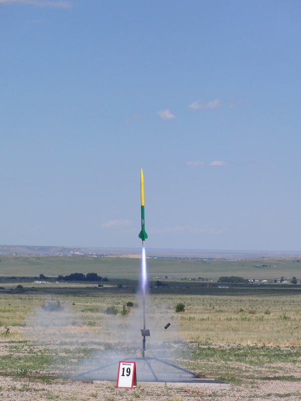
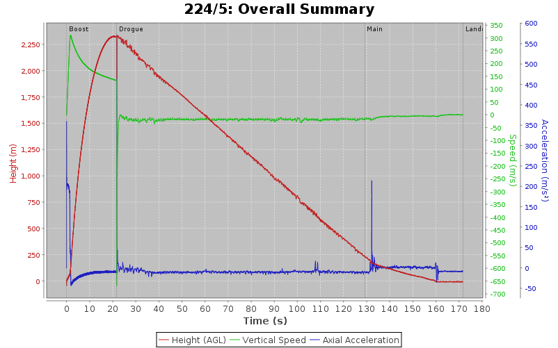
Anyhoo, somehow or other I’m now a Tripoli certified rocket scientist, with some launches and data to show for it:

Bunches of fun — and the data collection gives you an excuse to relive the flight over and over again while you’re analysing it. Who couldn’t love that? Anyway, as well as the five or six rocket flights I’ve done without collecting data (back in 2007 with a Rising Star, and after DebConf 10 at Metra with a Li’l Grunt), I’ve now done three flights on my Little Dog Dual Deploy (modified so it can be packed slightly more efficiently — it fits in my bag that’s nominally ok for carry-on, and in my bike bag) all of which came back with data. I’ve done posts on the Australian Rocketry Forums on the first two flights and the third flight. There’s also some video of the third flight:

But anyway! One of the things rocketeering focusses on as far as analysis goes is the motor behaviour — how much total impulse it provides, average thrust, burn time, whether the thrust is even over the burn time or if it peaks early or late, and so on. Commercial motors tend to come with stats and graphs telling you all this, and there are XML files you can feed into simulators that will model your rocket’s behaviour. All very cool. However, a lot of the guys at the Metra launch make their own motors, and since it tends to be way more fun to stick your new motor in a rocket and launch it than to put it on a testing platform, they only tend to have guesses at how it performs rather than real data. But Keith mentioned it ought to be possible to derive the motor characteristics from the flight data (you need to subtract off gravity and drag from the sensed acceleration, then divide out the mass to get force, ideally taking into account the fact that the motor is losing mass as it burns, that drag varies according to speed and potentially air pressure, and gravity may not be exactly aligned with your flight path), and I thought that sounded like a fun thing to do.

Unfortunately when I looked at my data (which comes, of course, from Bdale and Keith’s Telemetrum board and AltOS software), it turned out there was a weird warble in my acceleration data while it was coasting — which stymied my plan to calculate drag, and raised a question about the precision of the acceleration under boost data too. After hashing around ideas on what could be causing it on IRC (airframe vibration? board not tied down? wind?), I eventually did the sensible thing and tried recording data while it was sitting on the ground. Result — exactly the same: weird warbling in the accel data even when it’s just sitting there. As it turned out, it was a pretty regular warble too — basically a square wave with a wavelength of 100ms. That seemed to tie in with the radio — which was sending out telemetry packets ten times a second between launch and apogee. Of course, there wasn’t any reason for the radio to be influencing the accelerometer — they’re even operating off separate voltages (the accelerometer being the one 5V part on the board).

Hacking the firmware to send out telemetry packets at a different rate confirmed the diagnosis though — the accelerometer was reporting lower acceleration while the radio’s sending data. Passing the buck to Keith, it turned out that being the one 5V part was a problem — the radio was using enough current to cause the supply voltage to drop slightly, which caused all the other sensors to scale proportionally (and thus still be interpreted correctly), but the accelerometer kept operating at 5V leading to a higher output voltage which gets interpreted as lower acceleration. One brief idea was to try comparing the acceleration sensor to the 1.25V generated by the cpu/radio chip, but unfortunately it gets pulled down worse than the 3V does.

Fortunately this happens on more than just my board (though not all of them), so hopefully someone’ll think up a fix. I’m figuring I’ll just rely on cleaning up the data in post-processing — since it’s pretty visible and regular, that shouldn’t be too hard.

Next on the agenda though is trying some real-time integration with Google Earth — basically letting altosui dump telemetry data as normal, but also watching the output file for updates, running a separate altosui process to generate a new KML file from it, which Google Earth is watching and displaying in turn. I think I’ve got all the pieces for that pretty ready, mostly just waiting for next weekend’s QRS launch, and crossing my fingers my port HP Mini 2133 can handle the load. In any event, I hacked up some scripts to simulate the process using data from my third flight, and it seemed to work ok. Check out the recording:

BTW, if that sounds like fun (and if it doesn’t, you’re doing it wrong), now would probably be a good time to register for lca and sign up to the rocketry miniconf — there’s apparently still a couple of days left before early bird prices run out.

I saw a couple of things over the last couple of days about progressive taxation — one was a Malcolm Gladwell video on youtube about how a top tax rate of 91% is awesome and Manhattan Democrats are way smarter than Floridian Republicans; the other an article by Greg Mankiw in the New York Times about how he wants to write articles, but is disinclined too because if he does, Obama will steal from his kids.

Gladwell’s bit seems like almost pure theatre to me — the only bit of data is that during and after WW2 the US had a top marginal tax rate of just over 90% on incomes of $200,000 (well, except that WW2 and the debt the US accrued in fighting it isn’t actually mentioned). Gladwell equates that to a present day individual income of two million a year, which seems to be based on the official inflation rate; comparing it against median income at the time (PDF) gives a multiplier of 13.5 ($50,000/$3,700) for a top-tax bracket household income of $5.4 million ($2.7 million individual). I find it pretty hard to reason about making that much money, but I think it’s interesting to notice that the tax rate of households earning 5x the median income (ie $250,000 now, $18,500 then) is already pretty similar: 33% now, 35% then. Of course in 1951 the US was paying off debt, rather than accruing it… (I can’t find a similar table of income tax rates or median incomes for Australia; but our median household income is about $67,000 now and a household earning $250,000 a year would have a marginal rate between 40% and 45%, and seems to have been about 75% for a few years after WW2)

Meanwhile, Mankiw’s point comes down to some simple compound interest maths: getting paid $1000 now and investing it at 8% to give to your kids in 30 years would result in: (1) a $10,000 inheritance if it weren’t taxed, or (2) a $1,000 inheritance after income tax, dividend tax and estate tax — so effectively those taxes add up to a 90% tax rate anyway. If you’re weighing up whether to spend the money now or save it for your kids, you get two other options: (3) spend $523 on yourself, or (4) spend $1000 through your company. An inflation rate of just 2.2% (the RBA aims for between 3% and 4%) says (3) is better than (2), and if you want to know why evil corporations are so popular, comparing (3) and (4) might give it away…

An approach to avoiding that problem is switching to consumption taxes like the GST instead of income taxes — so you discourage people spending money rather than earning it. At first glance that doesn’t make a difference: there’s no point earning money if you can’t spend it. But it does make a huge difference to savings. For Mankiw’s example: 47.7% income tax ($1000 – $477 = $523) equates to 91.2% consumption tax (as compared to 10% GST); but your kids get $10,000 so can buy $5,230 worth of goods and still afford the additional $4,770 in taxes. As opposed to only getting $1,000 worth of goods without any consumption taxes.

The other side of the coin is what happens to government revenues. In Mankiw’s example, the government would receive $477 in the first year’s tax return, $1,173 over the next thirty years (about $40 per year), and $571 when the funds are inherited for a total of $2,221. That would work out pretty much the same if the government instead sold 30-year treasury bonds to match that income, and then paid off that debt once it collected the consumption tax. Since US Treasury’s are currently worth 3.75% at 30 years at the moment, that turns into $3,900 worth of debt after thirty years; which in turn leaves the government better off by $870. The improvement is due to the difference between the private return on saving (8%) versus the government’s cost of borrowing (3.75%).

Given the assumptions then, everyone wins: the parent, the kids, the government. It’s possible that would be the case in reality too; though it’s not certain. The main challenges are in the rates: if there’s a lot more saving going on (because it’s taxed less and thus more effective), then interest rates are liable to go down unless there’s a corresponding uptick in demand, which for interest rates means an uptick in economic activity. If Mankiw’s representative in being more inclined to work more in that scenario, that’s at least a plausible outcome. Similarly, if there’s a lot more government borrowing going on (because their revenue is becoming more deferred), then their rates might rise. In the scenario above, bond rates of 4.85% is the break even point in terms of a single 91.2% consumption tax matching a 47.7% tax rate on income and dividends and a 35% inheritance tax.

Not worrying about taxing income makes a bunch of things easier: there’s no more worries about earned income, versus interest income, versus superannuation income, versus dividend income, versus capital gains, versus fringe benefits, etc.

One thing it makes harder is having a progressive tax system — which is to say that people who are “worth” more are forced to contribute a higher share of their “worth” to government finances. With a progressive income tax, that means people who earn more pay more. With a progressive consumption tax, that would mean that people who spend more pay more — so someone buying discount soup might pay 10% GST (equivalent to 9.1% income tax), someone buying a wide screen tv might pay 50% (33% income tax) and someone buying a yacht might pay 150% (60% income tax). Because hey, if your biggest expenses are cans of soup, you probably can’t afford to contribute much to the government, but if you’re buying yachts…

One way to handle that would be to make higher GST rates kick in at higher prices — so you pay 10% for things costing up to $100, 50% for things costing up to $10000, and 150% for things costing more than that. The disadvantage there is the difference in your profit margin between selling something for $9,999 including 50% GST and $16,668 including 150% GST is $1.20, which is going to distort things. Why spend $60,000 on a nice car at 150% GST, if you can spend $9,999 on a basic car, $9,999 on electonics, $9,999 on other accessories, and $9,999 on labour to get them put together and end up with a nicer car, happier salesmen, and $20,000 in savings?

Another way to get a progressive income tax would be by doing tax refunds: everyone pays the highest rate when they buy stuff, but you then submit a return with your invoices, and get a refund. If you spend $20,000 on groceries over the year, at say 20% GST, then reducing your GST to 10% would be a refund of $1,667. If you spend $50,000 on groceries and a car, you might only get to reduce your GST to an average of 15%, for a refund of $2,090. If you spend $1,000,000 on groceries, a car, and a holiday home, you might be up to an average of 19.5% for a refund of just $4,170. Coming up with a formula that always gives you more dollars the more expenditure you report (so there’s no advantage to under reporting), but also applies a higher rate the more you spend (so it’s still progressive) isn’t terribly hard.

The downside is the paying upfront is harshest on the poorest: if you’re spending $2,000 a month on food it doesn’t help to know that $1,200 of that is 150% GST and you’ll get most of it back next year if you’re only earning $900 a month. But equally it wouldn’t be hard to have CentreLink offices just hand out $1,120 a month to anyone who asks (and provides their tax file number), and confidently expect to collect it back in GST pretty quickly. Having the “danger” be that you hand out $1,120 to someone who doesn’t end up spending $2,000 a month or more doesn’t seem terribly bad to me. And there’s no problem handing out $1,200 to someone making thousands a week, because you can just deduct it from whatever they were going to claim on their return anyway.

As I understand it, there’s not much problem with GST avoidance for three structural reasons: one is that at 10%, it’s just not that big a deal; another is that since it’s nationwide, avoiding it legally tends to involve other problems whether it be postage/shipping costs, delays, timezone differences, legal complexities or something else; and third is that because businesses get to claim tax credits for their purchases there’s paper trails at both ends meaning it’s hard to do any significant off-book work without getting caught. Increasing the rate substantially (from 10% to 150%) could end up encouraging imports — why buy a locally built yacht for $750,000 (150% GST) when you could buy it overseas for $360,000 (20% VAT say) and get it shipped here for $50,000? I don’t know if collecting GST at the border is a sufficiently solved problem to cope with that sort of incentive… On the other hand, having more people getting some degree of refund means it’s harder to avoid getting caught by the auditors if you’re not passing on the government’s tithe, so that’s possibly not too bad.

It appears the first draft of the linux.conf.au 2011 schedule (described by some as a thing of great beauty) is up as of this morning. Looks promising to me.

Of note:

• There’s lots of electronics-related talks (Arduino miniconf, Rocketry miniconf, Lunar Numbat, Freeing Production, “Use the Force, Linus”, All Chips No Salsa, e4Meter, Growing Food with Open Source, Lightweight Messaging, Misterhouse, and the Linux Powered Coffee Roaster). If you count mesh telephony too and don’t count the TBD slot, you can spend every day but Wednesday ensconced in hardware-hacking talks of one sort or another.
• There seems like reasonable female representation — Haecksen miniconf, LORE, HTML5 Video, Documentation, Intelligent Web, Incubation and Mentoring, Perl Best Practices, Project Managers, Growing Food with Open Source; so 7% of the miniconfs and 13% of the talks so far announced.
• Speaking of oppressed minorities, there’s also a couple of talks about non-Linux OSes: pf and pfsync on OpenBSD, and HaikuOS. Neato.
• Maybe it’s just me, but there seems to be a lot of “graphics” talks this year: GLSL, OptlPortal, Pixels from a Distance, X and the Future of Linux Graphics, HTML5 Video, Anatomy of a Graphics Driver; and depending on your point of view Print: The Final Frontier, Non-Visual Access, Can’t Touch This, and the X Server Development Process.
• The cloud/virtualisation stuff seems low-key this year: there’s Freeing the Cloud, Roll Your Own Cloud, Virtual Networking Performance, Virtualised Network Bandwidth Control, and ACID in the Cloud (that somehow doesn’t include an acid rain pun in the abstract). Of course, there’s also the “Freedom in the Cloud” and “Multicore and Parallel Computing” miniconfs which are probably pretty on point, not to mention the Sysadmin and Data Storage miniconfs which could see a bunch of related talks too.

And a bunch of other talks too, obviously. What looks like eight two-hour tutorial slots are yet to be published, maybe six more talks to be added, and three more keynotes (or given the arrangement of blank slots, maybe two more talks and four more keynotes). Also, there’s the PDNS on Wednesday, Penguin Dinner on Thursday, both over the river. And then there’s Open Day on Saturday, and an as yet not completely organised rocket launch sometime too…

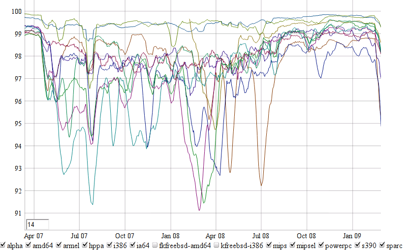
I’ve been playing with some graphing tools lately, in particular Dan Vanderkam’s dygraphs JavaScript Visualization Library. So far I’ve translated the RC bug list (the “official” one, not the other one) into the appropriate format, generated some numbers for an LD50 equivalent for bugs, and on Wouter’s suggestion the buildd stats.

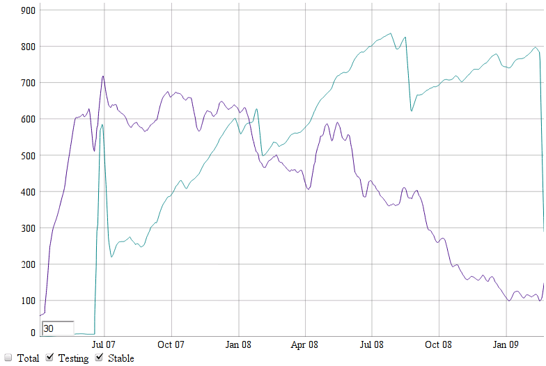
One of the nice things about the dygraphs library is it lets you dynamically play with the date range you’re interested in; and you can also apply a rolling average to smooth out some of the spikiness in the data. Using that to restrict the above graphs to the lenny development cycle (from etch’s release in April 2007 to lenny’s release in February 2009) gives some interesting stats. Remembering that the freeze started in late July 2008 (Debconf 8 was a couple of weeks later in August 2008).

RC bugs; first:

Not sure there’s a lot of really interesting stuff to deduce from that, but there’s a couple of interesting things to note. One is that before the freeze, there were some significant spikes in the bug count — July 2007, September 2007, November 2007, and April 2008, in particular; but after the freeze, the spikes above trend were very minor, both in size and duration. Obviously all of those are trivial in comparison to the initial spurt in bugs between April and June 2007, though. Also interesting is that by about nine months in, lenny had fewer RC bugs than the stable release it was replacing (etch) — and given that’s against a 22 month dev cycle, it’s only 40% of etch’s life as stable. Of course some of that may simply be due to a lack of accuracy in tracking RC bugs in stable; or a lack of accuracy in the RC bugcount software.

Quite a bit more interesting is the trend of the number of bugs (of all sorts — wishlist, minor, normal, RC, etc) filed each week — it varies quite a bit up until the freeze, but without any particular trend; but pretty much as soon as the freeze is announced trends steadily downward until the release occurs at which point there’s about half as many bugs being filed each week as there were before the freeze. And after lenny’s released it starts going straight back up. There’s a few possible explanations for the cause of that: it might be due to fewer changes being uploaded due to the freeze, and thus less bugs being filed; it might be due to people focussing on fixing bugs rather than finding them; it might be due to something completely unrelated.

An measure of development activity that I find intriguing is what I’m calling the “LD50” — the median number of days it takes a bug to be closed, or the “lethal dosage of development time for 50% of the bug population”. That’s not the same as a half life, because there’s not necessarily an exponential decay behaviour — I haven’t looked into that at all yet. But it’s a similar idea. Anyway, working out the LD50 for cohorts of bugs filed in each week brings out some useful info. In particular for bugs filed up until the lenny freeze, the median days until a fix ranged from as low as 40 days to up to 120 days; but when the freeze was declared, that shot straight up to 180 days. Since then it’s gradually dropped back down, but it’s still quite high. As far as I can tell, this feature was unique to the lenny release — previous releases didn’t have the same effect, at least to anywhere near that scale. As to the cause — maybe the bugs got harder to fix, or people started prioritising previously filed bugs (eg RC bugs), or were working on things that aren’t tracked in the BTS. But it’s interesting to note that was happening at the same time that fewer bugs were being filed each week — and indeed it suggests an alternative explanation for fewer bugs being filed each week: maybe people noticed that Debian bugs weren’t getting fixed as quickly, and didn’t bother reporting them as often.

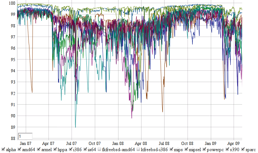
This is a look at the buildd “graph2”, which is each architecture’s percentage of (source) packages that are up to date, out of the packages actually uploaded on that architecture. (The buildd “graph” is similar, but does a percentage of all packages that are meant to be built on the architecture) Without applying the rolling average it’s a bit messy. Doing a rolling average over two weeks makes things much simpler to look at, even if that doesn’t turn out that helpful in this case:

Really the only interesting spots I can see in those graphs are that all the architectures except i386 and amd64 had serious variability in how up to date their builds right up until the freeze — and even then there was still a bit of inconsistency just a few months before the actual release. And, of course, straight after both the etch and lenny release, the proportion of up to date packages for various architectures drops precipitiously.

Interestingly, comparing those properties to the current spot in squeeze’s development seems to indicate things are promising for a release: the buildd up-to-dateness for all architectures looks like it’s stabilised above 98% for a couple of months; the weekly number of bugs filed has dropped down from a high of 1250 a week to about 770 at the moment; and the LD50 has dropped from 170 days shortly after lenny’s freeze to just under 80 days currently (though that’s still quite a bit higher than the 40 days just before lenny’s freeze). The only downside is the RC bug count is still fairly high (at 550), though the turmzimmer RC count is a little better at only 300, currently.

At the end of my previous post I mentioned some thoughts on dealing with more interesting initial states (\(q^0\)). We’ll define our initial state by choosing the amount of funds we’re willing to lose \(F\), and a set of initial prices \(0 < p_i(q^0) < 1\). Unless \(p_i(q^0) = \frac{1}{n}\) for all \(i\), we will be forced to set \(q^0_i > 0\) in some (possibly all) cases. We will treat this as implying a virtual payout from the market maker to the market maker.

The maximum loss, is then given by \(C(q^0) – \min(q^0_i) = F\) (since the final payout will be \(q_j – q^0_j\), the money collected will be \(C(q)-C(q^0)\), and \(C(q) \ge q_j\)).

If we wish to restrict quantities \(q_i\) to be integers, we face a dificulty at this point. Working from the relationship between \(p_i(q^0)\) and \(q^0_i\) gives:

\[ \begin{aligned}
p_i(q^0) & = \frac{e^{q^0_i/\beta}}{\sum_{j=1}^{n}{e^{q^0_j/\beta}}} \\
& = \frac{e^{q^0_i/\beta}}{e^{C(q^0)/\beta}} \\
& = e^{q^0_i/\beta – C(q^0)/\beta} \\
\beta \ln( p_i(q^0) ) & = q^0_i – C(q^0) \\
q^0_i & = C(q^0) + \beta \ln( p_i(q^0 ) )
\end{aligned} \]

Since \(C(q^0)\) is independent of \(i\), we can immediately see that the \(i\) with minimal \(q^0_i\) will be the one with minimal price. Without loss of generality, assume that this is when \(i=1\), then we can see:

\[ \begin{aligned}
F & = C(q^0) – q^0_1 \\
& = C(q^0) – \left( C(q^0) + \beta \ln(p_1(q^0)) \right) \\
& = – \beta \ln(p_1(q^0)) \\
\beta & = \frac{F}{\ln\left(p_1(q^0)^{-1}\right)}
\end{aligned} \]

In the case where \(p_i(q^0) = \frac{1}{n}\) is common for all outcomes this simplifies to the formula seen in the previous post.

Note that this is unlikely to result in a value of \(\beta\) that is particularly easy to work with. However simply rounding down to the nearest representable number works fine — since \(\beta\) is in direct proportion to the amount of funds at risk, this simply rounds down the amount of funds at risk at the same rate.

Likewise, keeping track of \(p_i(q)\) as an implementation choice will restrict us to rational prices, and thus likely irrational values for \(q_i\). However it’s likely we’d prefer to only offer precisely defined payoffs for precisely defined costs, even if only for ease of accounting. In order to deal with this, we can treat \(q_i = m_i(q) + g_i(q)\) where \(m_i(q) \ge q^0_i\) represents the (possibly increasing) virtual payout the market maker will receive, and \(g_i(q)\) are the (integer) payouts participants will receive. In particular, we might restrict \(q^0_i \le m_i(q) < q^0_i + 1\), so that we can calculate costs and payouts using the normal floor and ceiling functions and ensure any proceeds go to participants. This gets us very close to being able to adjust the outcomes being considered dynamically; so that we can either split a single outcome into distinct categories to achieve a more precise estimate, or merging multiple outcomes into a single category to reduce the complexity of calculations. If we look at changing the \(m \dotso n\)th outcomes from \(q\) into new outcomes \(m' \dotso n'\) in \(r\), then our presumed constraints are as follows. First, if this is the most accurate assignment between the old states and the new states we can come up with (and if it's not, use those assignments instead), then we need to set the payout for all the new cases to the worst case payout for the old cases: $$ g_{i'}(r) = \left\{ \begin{array}{l l} g_i(q) & \quad 1 \le i' < m \\ \max_{m \le i \le n}(g_i(q)) & \quad m' \le i' \le n \\ \end{array} \right. $$ Also, since we're not touching the prices for the first \(m-1\) outcomes, and our prices need to add up to one, we have: \[ \begin{aligned} p_{i'}(r) & = p_{i'}(q) \quad \forall 1 \le i' < m \\ \sum_{i'=m'}^{n'} p_{i'}(r) & = \sum_{i=m}^{n} p_i(q) \end{aligned} \] And most importantly, we wish to limit the additional funds we commit to \(\Delta F\) (possibly zero or negative), and thus \(C(r) = C(q) + \Delta F\). Using the relationship between \(p_i(r)\) and \(r_i\) again, gives: \[ \begin{aligned} C(r) & = r_i - \gamma \ln(p_i(r)) \\ & = m_i(r) + g_i(r) - \gamma \ln(p_i(r)) \\ \Delta F & = m_i(r) + g_i(r) - C(q) - \gamma \ln(p_i(r)) \\ \Delta F & \ge g_i(r) - C(q) - \gamma \ln(p_i(r)) \\ \Delta F & \ge \left\{ \begin{array}{l l} g_i(q) - C(q) - \gamma \ln(p_i(q)) & \quad 1 \le i < m \\ g_i(r) - C(q) - \gamma \ln(p_i(r)) & \quad m \le i \le n \\ \end{array} \right. \\ \Delta F & \ge \left\{ \begin{array}{l l} g_i(q) - C(q) - \left(q_i - C(q)\right) & \quad 1 \le i < m \\ \max_{m \le j \le n}(g_j(q)) - C(q) - \gamma \ln(p_i(r)) & \quad m \le i \le n \\ \end{array} \right. \\ \Delta F & \ge \left\{ \begin{array}{l l} -m_i(q) & \quad 1 \le i < m \\ \max_{m \le j \le n}\left( g_j(q) - \left( q_j - \beta \ln(p_j(q)) \right) \right) - \gamma \ln(p_i(r)) & \quad m \le i \le n \\ \end{array} \right. \\ \Delta F & \ge \left\{ \begin{array}{l l} -m_i(q) & \quad 1 \le i < m \\ \max_{m \le j \le n}\left( -m_j(q) + \beta \ln(p_j(q)) \right) - \gamma \ln(p_i(r)) & \quad m \le i \le n \\ \end{array} \right. \\ \end{aligned} \] Setting where \(\mu\) to be the modified outcome with maximum payout (that is, \(g_\mu(q) = \max_{m \le j \le n}(g_j(q))\), \(m \le \mu \le n\)) and \(\nu\) to be the least new price (so \(m' \le \nu \le n\) such that \(p_\nu(r) = \min_{m' \le j \le n'}(p_i(r))\)) lets us simplify this to: $$ \Delta F \ge -m_i(q) \quad \forall 1 \le i < m $$ and $$ \gamma \le \frac{\Delta F + m_\mu(q) + \beta \ln\left(p_\mu(q)^{-1}\right)}{\ln\left(p_\nu(r)^{-1}\right)} $$ Since \(m_i(q) \ge 0\), one simple approach to satisfying the inequalities is to simply drop the \(m_i(q)\) terms, giving: $$ \Delta F \ge 0 \quad \text{and} \quad \gamma \le \frac{\Delta F + \beta \ln(p_\mu(q)^{-1})}{\ln(p_\nu(r)^{-1})} $$ This has the drawback of not providing the maximum liquidity for the funds thought to be at risk, however.

Some additional notes on implementing Hanson’s Logarithmic Market Scoring Rule, based on David Pennock’s post from 2006.

Usage is to is to pick \(n\) distinct outcomes, such that exactly one will be true, and then to trade contracts that correspond with each outcome, so that if the outcome occurs the corresponding contract has a unit payoff, and otherwise is worthless. The market scoring rule provides a way for a market maker to set and update prices for the outcomes no matter how they might be bought and sold. While the market maker’s worst-case loss is limited to a fixed amount, \(F\), this is also the usual outcome.

The scoring rule uses a cost function, defined as:

\[ C(q) = \beta \ln\left( \sum_{i=1}^{n}{e^{\frac{q_i}{\beta}}} \right) \]

At any point, if event \(i\) occurs, the payoff owed to participants is \(q_i\). In order to achieve any given combination of payouts per outcome, a participant need simply pay \(C(q+\delta) – C(q)\) where \(\delta_i\) is the participant’s desired payout for event \(i\).

Prices thus vary non-linearly depending on both current payoff’s expected, and desired payoff. However a number of properties can be easily verified. First, the total payout for any event \(j\) is no more than \(C(q)\):

\[ \begin{aligned}
C(q) & = \beta \ln\left( \sum_{i=1}^{n}{e^{\frac{q_i}{\beta}}} \right) \\
e^{\frac{C(q)}{\beta}} & = \sum_{i=1}^{n}{e^{\frac{q_i}{\beta}}} \\
& \ge e^{\frac{q_j}{\beta}} \\
C(q) & \ge q_j
\end{aligned} \]

If we define the initial state, \(q^0\) by \(q^0_i=0\) for all \(i\), then \(C(q^0)=\beta \ln(n)\). \(C(q^0)\) is the maximum amount we can lose (since we will have received the remaining \(C(q)-C(q^0)\) from participants), and as such, we can define \(\beta\) in terms of the funds the marked maker can afford to lose, \(F\), as:

\[ \beta = \frac{F}{\ln(n)} \]

We can see that the cost of buying a payout of \(p\) in all scenarios (which we will denote as \(\delta = p\iota\), meaning \(\delta_i=p\) for all \(i\)) is exactly \(p\):

\[ \begin{aligned}
C(q+p\iota) & = \beta \ln\left( \sum_{i=1}^{n}{e^{\frac{q_i+p}{\beta}}} \right) \\
& = \beta \ln\left( \sum_{i=1}^{n}{e^{\frac{q_i}{\beta}} e^{\frac{p}{\beta}}} \right) \\
& = \beta \ln\left( \sum_{i=1}^{n}{e^{\frac{q_i}{\beta}}} \right) + \beta \ln\left( e^{\frac{p}{\beta}} \right) \\
& = C(q) + p \\
\end{aligned} \]

The instantaneous price of each contract is given by the derivative of the cost function, which works out to be:

\[ p_i(q) = \frac{\partial{C(q)}}{\partial{q_i}} = \frac{e^{\frac{q_i}{\beta}}}{\sum_{j=1}^{n}{e^{\frac{q_j}{\beta}}}} \]

We can directly observe from this that at any time the instantaneous prices of all the events will be between 0 and 1, and that they will sum to exactly 1. Furthermore, if we maintain a record of the values of \(C(q)\) (which represents the sum of funds received from participants and the maximum loss) and \(p_i(q)\), we can calculate \(q_i\):

\[ \begin{aligned}
p_i(q) & = \frac{e^{\frac{q_i}{\beta}}}{\sum_{j=1}^{n}{e^{\frac{q_j}{\beta}}}} \\
& = \frac{e^{\frac{q_i}{\beta}}}{e^{\frac{C(q)}{\beta}}} \\
& = e^{\frac{q_i}{\beta} – \frac{C(q)}{\beta}} \\
& = e^{\frac{q_i – C(q)}{\beta}} \\
\beta \ln\left( p_i(q) \right) &= q_i – C(q) \\
q_i &= C(q) + \beta \ln\left( p_i(q) \right) \\
\end{aligned} \]

Note that since \(0 \lt p_i(q) \lt 1\), then \(\beta \ln\left( p_i(q) \right) \lt 0\) and \(q_i \lt C(q)\) as expected.

If we partition the possible states into three disjoint sets, \(W\), \(L\) and \(I\), such that

\[ \delta_i = \left\{ \begin{array}{l l}
-c & \quad \mbox{ iff \(i \in L\) } \\
0 & \quad \mbox{ iff \(i \in I\) } \\
g & \quad \mbox{ iff \(i \in W\) }
\end{array} \right. \]

For notational convenience, we will write \(p_S(q) = \sum_{i \in S}{p_i(q)}\). If we set \(c > 0\) and \(C(q+\delta) = C(q)\), we then can determine \(g\):

\[ \begin{aligned}
C(q+\delta) & = C(q) \\
\beta \ln\left( \sum_{i=1}^{n}{e^{\frac{q_i+\delta_i}{\beta}}} \right)
& = \beta \ln\left( \sum_{i=1}^{n}{e^{\frac{q_i}{\beta}}} \right) \\
\sum_{i=1}^{n}{e^{\frac{q_i+\delta_i}{\beta}}}
& = \sum_{i=1}^{n}{e^{\frac{q_i}{\beta}}} \\
\sum_{i \in L}{e^{\frac{q_i-c}{\beta}}}
+ \sum_{i \in I}{e^{\frac{q_i}{\beta}}}
+ \sum_{i \in W}{e^{\frac{q_i+g}{\beta}}}
& = \sum_{i \in L}{e^{\frac{q_i}{\beta}}}
+ \sum_{i \in I}{e^{\frac{q_i}{\beta}}}
+ \sum_{i \in W}{e^{\frac{q_i}{\beta}}} \\
\sum_{i \in L}{e^{-\frac{c}{\beta}} e^{\frac{q_i}{\beta}}}
+ \sum_{i \in W}{e^{\frac{g}{\beta}} e^{\frac{q_i}{\beta}}}
& = \sum_{i \in L}{e^{\frac{q_i}{\beta}}}
+ \sum_{i \in W}{e^{\frac{q_i}{\beta}}} \\
e^{-\frac{c}{\beta}} \sum_{i \in L}{e^{\frac{q_i}{\beta}}}
+ e^{\frac{g}{\beta}} \sum_{i \in W}{e^{\frac{q_i}{\beta}}}
& = \sum_{i \in L}{e^{\frac{q_i}{\beta}}}
+ \sum_{i \in W}{e^{\frac{q_i}{\beta}}} \\
e^{-\frac{c}{\beta}} \sum_{i \in L}{p_i(q)}
+ e^{\frac{g}{\beta}} \sum_{i \in W}{p_i(q)}
& = \sum_{i \in L}{p_i(q)}
+ \sum_{i \in W}{p_i(q)} \\
e^{-\frac{c}{\beta}} p_L(q)
+ e^{\frac{g}{\beta}} p_W(q)
& = p_L(q) + p_W(q) \\
e^{\frac{g}{\beta}} p_W(q)
& = p_L(q) + p_W(q) – e^{-\frac{c}{\beta}} p_L(q) \\
e^{\frac{g}{\beta}}
& = 1 + \frac{p_L(q)}{p_W(q)} \left(1 – e^{-\frac{c}{\beta}} \right) \\
g & = \beta \ln\left( 1 + \frac{p_L(q)}{p_W(q)} \left(1 – e^{-\frac{c}{\beta}} \right) \right) \\
\end{aligned} \]

Since \(c > 0\), \(e^{-\frac{c}{\beta}} \lt 1\) and \(g\) is well defined and positive. This allows us to purchase \(c\iota\) and \(\delta\) at a total cost of \(c\), with the result that we end up losing \(c\) if an event in \(L\) occurs, we end up breaking even if an event in \(I\) occurs, and we gain \(g\) if an event in \(W\) occurs.

This provides a fairly straightforward way to calculate gains for a given cost using the prices, rather than the cost function directly.

Rather than choosing a particular amount to pay for a particular gain, it’s possible to determine how much it will cost to change the prices in a particular way. We might take the same sets, \(W\), \(I\), and \(L\) and instead decide to adjust the prices as follows:

\[ p_i(q+\delta) = p_i(q) \cdot \left\{ \begin{array}{l l}
y & \quad \mbox{ iff \(i \in L\) } \\
1 & \quad \mbox{ iff \(i \in I\) } \\
x & \quad \mbox{ iff \(i \in W\) }
\end{array} \right. \]

If we take \(p_W(q+\delta) = p_W(q) \cdot x = p_W(q) + \rho\) then since the prices always add to one, \(p_L(q+\delta) = p_L(q) \cdot y = p_L(q) – \rho\) and \(y = 1 – \frac{p_W(q)}{p_L(q)}(x-1)\)

The corresponding \(c\) and \(g\) values are then

\[ \begin{aligned}
x & = e^{\frac{g}{\beta}} \\
g & = \beta \ln(x) \\
& = \beta \ln\left( \frac{p_W(q) + \rho}{p_W(q)} \right) \\
& = \beta \ln(p_W(q+\delta)) – \beta \ln(p_W(q)) \\
\\
y & = e^{\frac{-c}{\beta}} \\
c & = -\beta \ln(y) \\
& = -\beta \ln\left( 1 – \frac{p_W(q)}{p_L(q)}(x-1) \right) \\
& = -\beta \ln\left( 1 – \frac{p_W(q)}{p_L(q)}\left( 1+\frac{\rho}{p_W(q)}-1 \right) \right) \\
& = -\beta \ln\left( 1 – \frac{\rho}{p_L(q)} \right) \\
& = \beta \ln\left( \frac{p_L(q)}{p_L(q) – \rho} \right) \\
& = \beta \ln(p_L(q)) – \beta \ln(p_L(q+\delta)) \\
\end{aligned} \]

Note that this assumes each price in \(W\) is multiplied by the same amount, and similarly for each price in \(L\). This also has the benefit that it maintains the relative prices within \(W\) and \(L\).

Obviously, \(I\) can be the empty set. The advantage of having outcomes in \(I\) is it allows participants to make their estimates conditional. For instance the statement “If X happens, Y will happen” should warrant a gain if “X and Y” happens, a loss if “X but not Y” happens, and no change if either “not X and not Y” or “not X but Y” happen.

This can also be used if a market may need to be cancelled. This may be done by having a “cancellation” outcome such that every action a participant may take results in that outcome being in \(I\). This prevents people from exiting the market place at a profit before the outcome is known, however.

Splitting and merging outcomes is an interesting possibility — if the price of “it will happen on Tuesday” is \(p\), then splitting that event into two events “it will happen on Tuesday morning” and “it will happen on Tuesday afternoon”, each with price \(p/2\) would allow more precise predictions. Having this happen dynamically (such as when \(p\) rises above a particular limit) would allow for precision only when it’s needed.

The drawback is that it may require an increase in \(F\) (but not always — once Tuesday has been split into morning and afternoon, splitting Wednesday as well can simply reuse the same extra funds). Having different “sized” regions may also require some care. Representation also becomes a possible issue. Some of the maths for handling this might also help with handling initial state \(q^0\) with different prices \(p_i(q^0) \ne p_j(q^0)\).

MathJax is pretty cool — it’s essentially a client-side JavaScript implementation of LaTeX, so you can write maths in ASCII, like “x^n + y^n = z^n”, surround it with dollar signs, and have it look like:

$$ x^n + y^n = z^n $$

And, of course, you can be more complicated if you like:

$$ C(\mathbf{q}) = b(\mathbf{q}) \log\left( \sum_i e^{\frac{q_i}{b(\mathbf{q})}} \right) $$

Inclusion in WordPress is easy: you unpack the MathJax beta on your website, add a “script” line so that the MathJax javascript is loaded, and it dynamically displays the maths when the page is loaded. It also manages to do it with real fonts, so you can select bits of the equations, and not have to deal with ugly images — oh, and it zooms nicely.

Of course, there’s a downside to having a client side script redisplay the formulas, and I suspect everyone reading via RSS will have already picked up on what it is…

Quite a long time ago I read a fascinating article on semiotics and user-interface design. My recollection is that it made the argument that computer user interfaces could be broken up into roughly three branches: “menus”, where you have a few options to choose between, and that’s it; “WIMP paradigm” where you’ve got windows, icons, menus and a pointer and can gesticulate to get things done; and “command oriented” where you type commands in to have things happen.

While the WIMP paradigm is obviously pretty good, it’s restricted by its “metaphoric” nature: you have to represent everything you want to do with a picture — so if you don’t have a picture for something, you can’t do anything with it. In effect, it’s reduces your interaction with computers to point-and-grunt, which is really kind of demeaning for its operators. Can you imagine if the “communication skills” that were expected of you in a management role in business were the ability to point accurately and be able to make two distinct grunting noises?

On the other hand, if your system’s smart enough to actually do what you want just based on a wave of your hand that is pretty appealing — it’s just that when you want something unusual — or when your grunts and handwaving aren’t getting your point across — you can’t sit down and explain what you want merely with more grunts and pointing.

Obviously that’s where programming and command lines come in — both of which give you a range of fairly powerful languages to communicate with computers, and both of which are what people end up using when they want to get new and complicated things done.

It’s probably fair to say that the difference between programming languages and command line invocations is similar to essays and instant messaging — programs and essays tend to be long and expect certain formulas to be followed, but also tend to remain relevant for an extended period; an IM or a command line invocation tends to be brief, often a bit abbreviated, and only really interesting exactly when it’s written. Perhaps “tweet” or “facebook status update” would be a more modern version of IM — what can I say, I’m an old fogey. In any event, my impression is that the command line approach is often a good compromise when point-and-grunt fails: it’s not too much more effort, but brings you a lot more power. For instance,

$ for a in *.htm; do mv "$a" "${a%.htm}.html"; done

isn’t a very complicated way of saying “rename all those .htm files to .html”, compared to first creating a program like:

#!/usr/bin/env python
import os
for name in os.listdir("."):
    if name.endswith(".htm"):
        os.rename(name, name[:-4]+".html")

and then running it. And obviously, one of the advantages of Unix systems is that they have a very powerful command line system.

In any event, one of the things that strikes me about all the SaaS and cloud stuff is that there really isn’t much a linguistic equivalent to the command line for the web. If I want to do something with gmail, or flickr, or facebook I’m either pointing and grunting, or delving deeply into HTML, javascript, URLs, REST interfaces and whatever else to make use of whatever arbitrary APIs happen to be available.

A few services do have specialised command line tools of course — there’s GoogleCL, various little things to upload to flickr, the bts tool in devscripts to play with the Debian bug tracking system, and so forth.

But one of the big advantages of the web is that you aren’t meant to need special client side tools — you just have a browser, and leave the smarts on whichever web server you’re accessing. And you don’t get that if you have to install a silly little app to interface with whichever silly little website you happen to be interested in.

So I think there ought to be a standard “command line” API for webapps, so that you can say something like:

$ web www.google.com search -q='hello world'

to do a Google search for ‘hello world’. The mapping from the above command line to a URL is straightforward: up until the option arguments, each word gets converted into a portion of the URL path, so the base url is http://www.google.com/search, and options get put after a question mark and separated by ampersands, with regular URL quoting (spaces become plusses, irregular characters get converted to a percent and a hex code), in this case ?q=hello+world.

The obvious advantage is you can then use the same program for other webapps, such as the Debian BTS:

$ web bugs.debian.org cgi-bin bugreport.cgi --bug=123456 --mbox=yes
From mech...@...debian.net Tue Dec 11 11:32:47 2001
Received: (at submit) by bugs.debian.org; 11 Dec 2001 17:32:47 +0000
Return-path: 
Received: from gent-smtp1.xs4all.be [195.144.67.21] (root)
	by master.debian.org with esmtp (Exim 3.12 1 (Debian))
	id 16Dqlr-0007yg-00; Tue, 11 Dec 2001 11:32:47 -0600
...

It obviously looks cleaner when you use the shorter url (web bugs.debian.org 123456), although due to the way the BTS is setup, you also lose the ability to specify things like mbox format then.

Of course, web pages are in all sorts of weird formats, too: having Google’s HTML and javascript splatter all over your terminal isn’t very pleasant, for instance. But that’s what pipes are for, right?

$ web chart.apis.google.com chart --cht=p3 \
    --chs=400x150 --chd=t:2,3,5,10,20,60 \
    --chl='Alice|Bob|Carol|Dave|Ella|Fred' | display

It’d probably be interesting to make “web” clever enough to automatically pipe images to display and HTML to firefox and so on, depending on what media type is returned.

Obviously you can use aliases just like you’d use bookmarks on the web, so saying:

$ alias gchart='web chart.apis.google.com chart'
$ alias debbug='web bugs.debian.org cgi-bin bugreport.cgi'

lets you type a little less.

Anyway, I think that makes for a kind-of interesting paradigm for looking at the web. And the “web” app above is pretty trivial too — as described all it does is convert arguments into a URL according to the given formula.

Things get a little more interesting if you try to make things interactive; a webapp that asks you your name, waits for you to tell it, then greets you by name is made unreasonably difficult if you try to do it on a single connection (with FastCGI and nginx for instance, the client has to supply the exact length of all the information you’re going to send before it will receive anything, and if you don’t know what you’re going to need to send up front…). Which means that so far my attempts to have web localhost bash behave as expected aren’t getting very far.

The other thing that would be nice would be passing files to remote web apps — being able to say “upload this avi to youtube” would be more elegant as web youtube.com upload ./myvideo.avi than web youtube.com upload <./myvideo.avi, but when web doesn’t know what “youtube” or “upload” actually means, that’s a bit hard to arrange. After all, maybe you were trying to tell youtube to do the uploading to your computer, and ./myvideo.avi was where you wanted it to end up.

Anyway. Thoughts appreciated.

My previous post apparently didn’t do the economics for the resource rent analysis quite right — it seems that the idea is a cleverer company would be able to use the resource rent tax to find cheaper sources of funding, which changes things…

The idea then would be that you start your mining project seeking 60% in risky funding (they get whatever profits you make and the totality of the loss), and 40% in risk-free funding (they get the same return as they would if they invested in government bonds, whether the project succeeds or fails). That’s as opposed to the current approach of seeking 100% in risky funding.

So say you’ve raised $5B. You spend your $5B doing surveys, setting up your mine, etc. Failure here means you declare bankruptcy and the government gives you enough money to pay back the $2B of risk-free investment, plus interest, presuming the Greens don’t have their way. On the other hand, your mine might be a success, and you might, eg, start getting $1.5B in revenue, against $500M in expenses. At this point you first have to pay your “super profit” tax, which is, apparently 40% of:

• gross receipts: $1.5B
• less depreciation: assuming 20 year expected life, 5% of 5B = $250M
• less running expenses: $500M
• less “normal return” on debt/equity: 6% of $5B = $300M
• totalling: $450M

So $180M on resource rents. You then pay corporate income tax of 30% (eventually 28%) of:

• gross receipts: $1.5B
• less depreciation: assuming 20 year expected life, 5% of 5B = $250M
• less running expenses: $500M
• less resource rent: $180M
• totalling: $570M

So $171M ($159.6M at 28% in 2014 or so).

You then pay the risk-free return to your risk-free investors, which is 6% of $2B or $120M. (Actually, this might be tax deductible too)

So after paying expenses ($500M), resource rents ($180M), income tax ($171M) and the risk-free dividend ($120M), your $1.5B of earnings is down to $529M. Issuing all that to your risky investors, gives an annual return of 17.63%, fully-franked.

That compares to doing things the current way as follows: you raise $5B of risky investment; your mine succeeds and makes $1.5B in revenue, against $500M in expenses. You just pay company tax at 30% after expenses and depreciation, so that’s 30% of $750M, or $225M. That leaves you $775M to pay in dividends, which is an annual return of 15.5%, fully-franked.

That, obviously, is an entirely convincing investment. It relies on the government refunding the $2B of “risk-free” investment in the event that the mine falls apart, though — which, as I understand it, is the part of the plan the Greens oppose. But otherwise, the above’s fairly plausible.

The difference in those sums — profit rising from 15.5% to 17.63% is due to the level of depreciation in the above sums. If those formulas for calculating the rent and company taxes are correct, then your return on investment increases by two-thirds of your annual depreciation compared to the initial investment and decreases by a fifth of the risk-free rate. In the above case, annual depreciation was 5% of the entirety of the initial investment, and the risk-free rate was 6%, which implies an improvement of 2/3*5%-6%/5 which is the 2.13% we saw.

In reality, you’d probably need to offer a higher return to your “risk-free” investors — because if you didn’t, they’d probably just by bonds directly from the government in the first place. And if I’m not mistaken you still need to repay the principle for your risk-free investors over the life of your mind. So hopefully that simply evens out in the end.

There’s not a lot of difference in that scenario to having the government borrow enough to maintain 40% ownership in every mining operation in Australia. They’ll then receive 40% of the after-tax profits, and have to pay interest on their borrowings at the long term bond rate, which would mean (in the above example) getting $225M in company tax, then $310M in franked dividends, then paying out $120M in interest costs for a total of $415M extra per-annum. That’s more than the total of $351M in receipts in the above example, I think due to the depreciation deduction in the resource rent tax calculation.

Mechanically, there’s a few differences: the company has to gain two sorts of investment (risky shares and risk-free bonds, for instance), if it fails it has to go to a lot more trouble to pay back the risk-free investors (getting the tax office to issue a refund in cash), and the government gets to keep it mostly off its books (doesn’t have to raise funds directly, investment losses turn into tax refunds).

In any event, that should make it easier for mining companies to raise funds — they only need to raise 60% of the amount at the risky level, for the same return they previously offered.

I don’t see anything stopping you from being tricky and doing a two stage capital raising: raising $3B of risky funds to do exploration; and if that fails repaying your investors 40% ($1.2B) of their capital — then doing the risk-free fund raising to get enough cash to start production. The initial fund raising then has a chance at a 17% ongoing return, or a 60% loss — compared to currently having a chance at a 15% return or a 100% loss. Again, that should make it easier to raise funds for new projects.

On the other hand, I also still don’t see anything stopping you from transferring your profits. Say you’re a public investment company. You’ve got plenty of money from offering superannuation products or what not, and you want to get into mining because you hear it gives a high return for your investors. So you allocate a few billion to start a mining company, which does some prospecting and opens a mine. That works out, and it starts making super profits. You decide you want to reduce your tax, and get more dividends. So instead of having one privately held subsidiary mining company, whose balance sheet looks like:

• Revenue: $1500M
• Expenses: $500M
• Resource rent tax: $180M
• Company tax: $171M
• Dividends: $649M

you decide to invest in a transport company as well. Hopefully one that’s already making a decent profit, but paying a bit more than market value works too. You then have them make an agreement that the mine will exclusively use your transport company for the next 10 or 20 years, for whatever excuse satisfies appropriate laws. Then have the transport company seriously jack up the price. Your balance sheets should then look like:

And voila, your resource rent tax has been reallocated to your dividends (except for the 30% that goes to company tax, of course). It doesn’t have to be a transport company, either — any private company that you can buy outright, that isn’t hit by the resource tax, and that you can find some excuse to make your exclusive supplier of a necessary product/service will do fine. And even better, as far as I can see, even when you get rid of all the resource rent proceeds the government was hoping for from your mine, they’ve still covered 40% of your initial risk…